
Genre: Self-help Book, Non-Fiction
Author: Jordan Ellenberg
Book: How Not to Be Wrong: The Power of Mathematical Thinking (Buy the Book)
Summary
How Not to Be Wrong is a consumer-friendly briefing of a few mathematical concepts and their importance to everyday life. Throughout this work, Ellenberg doesn’t talk about complicated formulas or equations, but instead, the fundamentals of mathematical thinking.
He argues that math isn’t just indefinite lists of computations, but that the seemingly endless computations we do in school are like training for life’s challenges – he likens this to an athlete practicing endless training drills, though he never uses them directly in the games. Once you know math, it’s like wearing a pair of x-day glasses that allow you to identify underlying structures and patterns in everyday life.
Knowing math provides you with a tool to gain a deeper understanding of the world around you. You can use mathematical thinking to get problems of commerce, politics and even theology right. When students ask:
“when am I ever going to use math in real life?”
they should be referred to this book.
Ellenberg breaks his book into 5 main sections corresponding to 5 broad themes in mathematics and its applications: linearity, inference, expectation, regression and existence.
In the first section, he discusses an assumption that many people make: that relationships between inputs and outputs are always linear. Through a few examples, he describes the pitfalls of this often-incorrect assumption. More of a good thing is not always better, and the scale at which you observe relationships changes their linearity.
In the second section, he discusses inference – the process of drawing conclusions about a broader population by observing some smaller set of samples. While many extremely powerful statistical tools rely on inference, they require a deep understanding of inference as misuse frequently leads to extremely incorrect conclusions.
In the third section, he introduces the concept of expected value – not the value that you expect if you engage in one uncertain event but the average value that you would expect given a large number of chances. Additionally, it is important not only to consider the most likely outcome but incorporate all possible outcomes into your analysis. Lastly, given a large number of chances, improbable things become probable.
In the fourth section, he discusses regression to the mean. Regression to the mean occurs in many fields including business, sports, genetics and others. Often times, the exceptional performance of the best players and the worst players is a function of random fluctuations. Over time, these effects wear out, and their performance tends to more closely resemble the broader population.
In the fifth section, he discusses existence – a combination of seemingly paradoxical realities and a few abstract mathematical concepts such as set theory and non-traditional coordinate systems. Most notably, he explores the difficulty in fairly understanding public opinion and the conclusion that in many circumstances it simply does not exist.
Ellenberg closes the book by summarizing the key findings. Chief among these is the notion that there is structure in the world, and math allows us not only to understand that structure but make the best possible decisions based on our observations.
Although the book is titled How Not to be Wrong, Ellenberg does not assert that knowing math guarantees you will always achieve the most desirable outcome – math gives us a principled method of being uncertain. Mathematical certainty is not the same as the everyday convictions we have become accustomed to thinking of as certainties.
Overall, How Not to be Wrong is an engaging read that helps the reader understand important concepts. Ellenberg’s abundant use of relatable and interesting stories makes the concepts memorable, and the structure of the book makes the content digestible.
The mathematical concepts explored here are relatively basic, though a reader should have a basic understanding of geometry, algebra, probability and data visualizing to gain the most utility from this book.
INTRODUCTION
Abraham Wald was an Austrian mathematician during World War II. He was a part of the high powered “Statistical Research Group” which used math to make wartime recommendations to the military. One of his most famous recommendations was the case of the “missing bullet holes”. When asked to determine where to reinforce the armor on fighter jets, he inspected the placement of bullet holes on fighter jets that returned from combat.
Upon inspection, he counterintuitively recommended reinforcing the armor where there were few bullet holes, while the generals had instead expected him to tell them how much more armor was needed in the places with many bullet holes. While there were numerous equations involved in computing the optimum armor distribution, the underlying thinking was clear: Wald assumed planes were hit with relatively even distribution, so the areas of the planes with few holes weren’t getting hit less, but instead, hits to those areas were lethal.
Therefore, armor should be reinforced where the holes were scarce, not where the holes were plentiful. In this case, mathematical thinking is
about asking yourself what assumptions you are making and what the implications of those assumptions might be. The Air Force generals incorrectly assumed that the planes coming back were representative of all planes in the war, but Wald knew that it was a biased sample as these were only the planes that survived. He was able to look past the context of planes, bullets and war to see the underlying structure of the problem: a phenomenon called survivorship bias.
Wald’s recognition of the generals’ incorrect assumption may not seem to resemble the math we are accustomed to. It does not include complex equations, trigonometric identities or calculus. It probably just seems like common sense, and that is the exact point of this story: all math starts from a point of common sense. Math is an extension of common sense by other means. In Ellenberg’s words:
“Math is like an atomic-powered prosthesis that you attach to your common sense, vastly multiplying its reach and strength.”
Math offers rigorous structure to common sense that allows you to accurately reach beyond the obvious. However, it is important to maintain your common sense as you dive deep into the abstract reaches of math – it is this “interplay between abstract thinking and our intuitions about quantity, time, space, motion, behavior and uncertainty” that allows math to work.
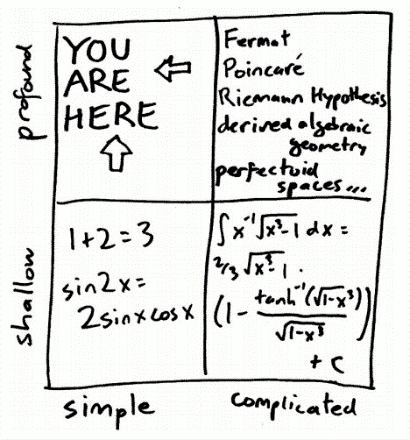
When considering the various types of mathematical facts, Ellenberg segments them into four categories based on a 2 x 2 matrix (left). On one axis, facts are categorized by the complexity of the computations involved: some are simple, while others are more complicated.
On the second axis, facts are categorized by how meaningful the contribution is: some are shallow, while others are profound. Contemporary professional mathematicians attempt to spend most of their time in the complicated-profound quadrant; however, there are many interesting observations in the simple- profound quadrant. How Not to Be Wrong focuses on the simple- profound quadrant.
Ellenberg breaks his book into 5 main sections corresponding to 5 broad themes in mathematics: linearity, inference, expectation, regression and existence. In each section, he offers digestible examples of the usefulness of each concept as well as common pitfalls and applications for these concepts. In each section, he offers digestible examples of the usefulness of each concept as well as common pitfalls and applications for these concepts.
PART 1: LINEARITY
In this section, Ellenberg describes numerous cases in which challenging the assumption of linearity can lead to interesting findings. Sometimes common phenomena are assumed to be linear but are, in fact, non-linear. In other cases, phenomena are assumed to be non-linear but can, in fact, be considered linear when viewed on a different scale. Understanding when to apply linear and non-linear thinking leads to useful insights.
Some things are non-linear
There is a common fallacy: “if a thing is good, more of it must be better.” This fallacy is an example of assuming that a non-linear phenomenon is in fact linear. Ellenberg debunks this fallacy using a blog entry authored by the Cato Institute that condemned taxation and government provided social benefits based on this principle. In the post titled: “Why is Obama Trying to Make America More Like Sweden when Swedes Are Trying to Be Less Like Sweden?” Daniel J. Mitchel argues that Swedishness (in this context defined by the amount of government funded social welfare) is obviously bad, as even the Swedes have recognized that being less Swedish would lead to higher prosperity. His vision was something like the curve on the left. In reality, the issue is not linear and the reality looks something like the middle curve.
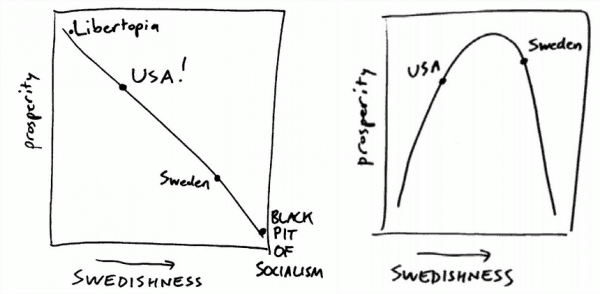
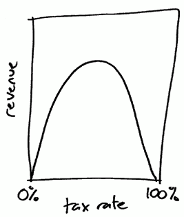
This is an example application of the Laffer Curve – a simple economic model developed by Arthur Laffer. The Laffer Curve looks something like the curve on the right. At a 0% tax rate, there would obviously be no tax revenue. Likewise, at a 100% tax rate, people would not have any incentive to work for pay, and there would again be no tax revenue.
The optimal tax rate lies somewhere in the middle. While the exact tax rate or level of “Swedishness” that will maximize tax revenue or national prosperity is context-specific and still up for debate, simple statements like “more tax is always good” or “everyone needs to be less Swedish, just look at the Swedes” are not accurate.
Sometimes non-linear things can actually be linear
Though curves may always appear to either be linear or non-linear, it is important to realize that the distinction between linear and non-linear is not always clear depending on the scale at which the curve is viewed. At small scales, non-linear curves can be approximated by small linear segments.
Archimedes drew on this concept when he developed the method of exhaustion to calculate the area of a circle. At the time, there was no way to calculate the area of a circle because of its non-linear curvature. However, by drawing polygons using straight lines and known angles (areas which could be computed), he could estimate the area of the circle.
The method goes something like this. Start with a circle with a radius of 1 and draw a square inside of it (the inscribed square) where all 4 corners touch the circle at one point. This square can be divided into 4 equal right triangles, and by the Pythagorean Theorem, the length of the sides of the square can be computed to be equal to the square root of 2.
From there, the area of the square can be computed to be 2. Next, another square is drawn outside of the circle (the circumscribed square) and this one also touches the circle at only 4 points. The length of each side of this square is 2, and the area of this square is therefore 4. From this, we know the area of the circle is more than 2 but less than 4. This method can be extended to an octagon, then a 16-gon, and so on and so forth 15 times.
At this point, the resultant 65536-gon looks so similar to the circle that it doesn’t matter if it’s a circle or a polygon, the areas will be so close that the difference doesn’t matter for any practical purpose. As this process goes on to infinity, the two become the same.
Numerous other interesting phenomena arise as we delve into the infinite (or practically speaking, small enough that the calculable mirrors the behavior of the infinite). This similarity between the infinite and small enough or numerous enough to mimic the infinite is the basis of calculus.
PART 2: INFERENCE
Inference is the basis of many statistical methods. Simply stated, it is the assertion that conclusions about full sets of data (or populations) can be drawn by observing a randomly selected subset of that data (samples). Inference is a very powerful statistical tool that has led to many discoveries in traditional fields such as science, engineering, finance and medicine, but also in surprising places such as theology.
However, like other mathematical tools, when used incorrectly, statistical tests rooted in inference will reject true conclusions and fail to reject untrue hypotheses. While using inference as a basis for decision making (whether formally through statistics or informally through crude observation) it is important to understand that improbable things happen all the time.
Given enough chances, improbable becomes probable
Ellenberg uses a few stories to illustrate that given enough chances, improbable things happen often. The parable of the Baltimore stockbroker goes something like this. One day, you receive a stock tip from a broker that says a certain stock will rise in the next week. A week passes and that stock does in fact rise.
The next week you receive another tip that a different stock will fall, and a week later, sure enough, the stock falls. 10 weeks pass, and you receive 10 tips that correctly predict the movement of 10 stocks. By the 11th week, you are so impressed by his stock-picking prowess that you invest your money. However, these 10 picks were not evidence of a prescient stockbroker, you were the victim of a scam.
If you look from the stock broker’s point of view it becomes much clearer how he actually picked correctly 10 times in a row. From the stockbroker’s point of view, the story goes something like this. Suppose any given week there is a 50% chance that a given stock rises. Then, over the course of 10 weeks, there is a 1/1024 chance that 10 random picks would be correct. The first week, he sends his picks to 10,240 people – 5,120 get a letter that says the stock will rise, and 5,120 get a letter that says the stock will fall.
Given the 50% chance that the stock will rise, 5,120 people will have received a correct tip. When the next week rolls around, he sends his newsletter to the 5,120 who received the correct pick, this time sending 2,560 tips that say rise, and 2,560 tips that say fall. He repeats this for 10 weeks and by the 11th week, there are 10 people who received 10 correct stock picks in a row. The important thing to consider here is:
how many chances did the stockbroker have to get these picks correct?
On the receiving end of his newsletters, it is impossible to know. Therefore, it is unwise to believe his performance was the result of some special financial foresight.
This idea is not limited to the realm of parables. Ellenberg describes numerous real world examples of this phenomenon. Throughout the 20th century, some mathematically inclined Rabbi decided to search the Torah for hidden messages. They employed a technique called “equidistant letter sequence” or ELS to interpret the text. ELS goes something like this. Suppose you have a text that says: DON YOUR BRACES ASKEW. A 5 letter ELS would reveal the hidden word: DUCK, by extracting every fifth letter.
Upon inspection, the Rabbi found numerous hidden messages ranging from the word TORAH to the death dates of famous Rabbi. However, it is important to realize that just like the Baltimore stockbroker, the number of chances matter. The Torah has 304,805 letters in the text. Upon further investigation of the methods and similar studies revealing hidden messages in other texts such as War and Peace, the Rabbis’ findings were ultimately rejected.
The law of large numbers
In short, the law of large numbers roughly states that it becomes increasingly more unlikely to see inaccurate results as the number of experiments increases. Coin flips are a great example of the law of large numbers. If someone were to flip 10 coins and saw 8 heads and 2 tails, it does not mean the coin is unbalanced.
However, it is (for practical purposes) impossible to flip 10,000 balanced coins and observe 80% heads due to the law of large numbers. In fact, Abraham de Moivre calculated that it is more unlikely to flip 54% heads in 1,000 tries than it is to flip 60% heads in 100 tries.
Carelessly applied statistics leads to incorrect conclusions
When trying to draw inferences about systems using mathematics, we are often presented with yes or no questions. However, when analyzing data to validate your hypothesis, the data must not only be consistent with your theory but also inconsistent with the negation of your theory. For example, if I believe I have telekinetic powers to make the sun rise, the sun rising when I tell it to does not prove my hypothesis. The sun must also fail to rise if I don’t use my telekinetic powers.
The second statement – that the sun must fail to rise if I don’t use my telekinetic powers – is the null hypothesis. Null hypothesis testing basically says: 1) suppose your null hypothesis is true and let p be the probability under that hypothesis that you observe the results that you have 2) if p (also called the p value) is small, then your results are statistically significant (ie, it is sufficiently unlikely that you would observe the results that you have if your null hypothesis is true), if p is large, then the null hypothesis cannot be ruled out.
The null hypothesis test or p value test has become a standard among medical, scientific and social science publications, but it is important to understand the limitations of this approach. The generally accepted convention is to select a p value of 0.05.
In other words, there is a 1 in 20 chance that a researcher would observe these results if the null hypothesis is true. In most cases, researchers have sufficient reason to believe their hypothesis before testing it, so the 1 in 20 odds are enough. However, we’ve seen with the Baltimore stock broker that improbable things happen all the time given enough chances.
There are many ways the p value test can be misused. First, experiments without sufficient theoretical framework can be misinterpreted. Ellenberg gives two examples of this. In 2009, a group of researchers published a satirical paper (though the data and analysis were real) in which they showed statistically significant evidence that a dead salmon could read emotions.
When various pictures where shown to the salmon, certain voxels (brain waves observed through fMRI scans) lit up. Of course, these correlations were nothing more than random noise – with the vast amount of data it was highly likely that some of the voxels correlated with the timing of the pictures that were shown.
In a more broadly published field of study, Haruspex (people who sacrifice sheep then interpret the entrails to predict the future) execute numerous experiments and publish the ones that work. Of course, given what we already know about the p value, we expect that 1 in 20 experiments will show statistically significant results. However, hundreds of these papers are published in The International Journal of Haruspicy.
These two stories do not mean that all papers or scientific conclusions based on p value testing should not be trusted, just that scientists and researchers should be careful to present sufficient theoretical framework to form a causal argument and employ additional tools such as multiple comparisons analysis to validate surprising results.
A second way in which p value tests can be misused is when they are underpowered. Small results may not show up on p value tests. An example of this is the “hot hand” myth in basketball. The “hot hand” says that sometimes players display short bursts of greatness in which they seemingly cannot miss a shot.
After many rigorous statistical analyses sought to prove it did not exist – and indeed they could not detect it – a group of computer scientists showed that the statistical tests were simply not high power enough to detect the effect, even if it was real. They did so by simulating players’ seasons but explicitly adding in sequences where the players possessed the hot hand. But even in these sequences, the statistical tests were unable to show a result.
The phrase “statistically significant” is also misleading. Really, this phrase simply means an effect exists, not necessarily that the effect is important, large or meaningful. A third way, therefore, that statistical tests may be misused is overstating the meaningfulness of statistically significant results. An example of this occurred in 1995 when the UK Committee on Safety of Medicines released a “Dear Doctor” indicating that a certain type of birth control doubled the risk of thrombosis.
This “statistically significant” effect turned out not to be very meaningful or important as the risk of thrombosis was already very small to begin with. This letter led to a dramatic reduction in the number of women taking birth control, naturally leading to a spike in the number of unplanned pregnancies (26,000) and abortions (13,600). When the dust settled, the researchers who released the study said the additional risk presented by the new birth control may have, at most, taken the life of one woman.
The stories of the British birth control scare, the “hot hand” myth, and dead fish reading minds all show the importance of using statistical tools correctly. Particularly, it is important to 1) choose an appropriate test 2) understand what you can and cannot test for and 3) understand the context and other factors that may be influencing your outcomes.
PART 3: EXPECTATION
Expected value is a commonly used metric when dealing in uncertainty. It is essentially the average value that you would expect to see over a large number of occurrences.
If gambling is exciting, you’re doing it wrong
When deciding whether or not to play the lottery, you should consider the expected value of the lottery ticket. Expected value can be calculated by multiplying each potential outcome by the probability of that outcome, and summing up these numbers for all of the potential outcomes.
For example, suppose you have a lottery ticket with a 1/10,000,000 chance of winning the $6 million dollar jackpot, and a 9,999,999/10,000,000 chance of being worthless. The expected value of that ticket would be 1/10,000,000 × $6,000,000 + 9,999,999/10,000,000 × $0 = $0.60. That does not mean you expect the single ticket to be worth $0.60, but instead, if you purchased a large number of tickets, say 10 million, you would expect the average value of those 10 million tickets to be $0.60.
Normally, lottery tickets are priced such that the expected value of the ticket is less than the purchase price of the ticket in order to ensure the state makes money. Due to this expected value calculation, the lottery is usually not a good bet.
In 2004, Massachusetts decided to change their lottery system in order to increase participation. Instead of the traditional lottery where the jackpot continued to accumulate week to week until someone correctly guesses the 6 ball combination to win the jackpot, Massachusetts introduced a new game called Cash Windfall.
In Cash Windfall, the jackpot would continue to grow week to week as long as no one guessed the correct 6 ball combination; however, the difference came in the weeks that the jackpot reached a designated size: the massive jackpot triggered a roll down. During a roll down, it was not necessary to guess the 6 ball combination in order to win the jackpot. Players who correctly guessed 5 of 6, 4 of 6, and even 3 of 6 numbers would split the jackpot in various proportions, therefore raising the chances of success and increasing participation in the lottery.
A group of MIT students studying the lottery for class discovered an interesting phenomenon – during the rolldown weeks, the expected value of a lottery ticket exceeded the purchase price of a lottery ticket. Massachusetts had inadvertently designed a game that was, in fact, a good bet. Based on the expected values of each winning combination, the expected value of a $2 ticket was $5.54 as illustrated below.
| Prize | Chance of Winning | Expected number of winners | Roll Down Allocation | Roll– Down per Prize | Expected Value Calculation | Expected Value |
| Match 5 of 6 | 1 in 39,000 | 12 | $600 K | $50,000 | 1/39,000 × $50,000 | $1.28 |
| Match 4 of 6 | 1 in 800 | 587 | $1.4 M | $2,385 | 1/800 × $2,385 | $2.98 |
| Match 3 of 6 | 1 in 47 | 10,000 | $600 K | $60 | 1/47 × $60 | $1.28 |
| Total Expected Value: | Match 5 + Match 4 + Match 3 | $5.54 |
The MIT students, along with a few other betting clubs, placed massive bets – and won big – during the roll down weeks for the duration of the Cash Windfall game. The lesson here is that while expected value is not the value you can expect while placing one bet, by invoking the law of large numbers, expected value can be realized as the average value of a bet when a sufficiently large number of bets are placed.
Risk/waste reduction is not always beneficial
There is a Laffer style tradeoff between reducing risk or eliminating waste, and the cost of reducing risk or eliminating waste. This means that if you spend too little effort reducing risk, the risk will be large and will hurt you. Conversely, however, spending too much effort reducing risk, the effort spent reducing the risk will cost you more than taking the risk would have.
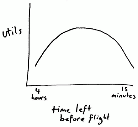
“If you never miss a plane, you’re spending too much time at the airport.” To most people, this quote seems counterintuitive: if I miss my plane, won’t I spend more time at the airport? The answer to this question is maybe. In order to compute the tradeoff, economists use the standard measurement of utils to measure the utility of commodities such as time or money.
This is necessary as the value of the time spent getting to the airport early, may not be as valuable as the time lost at the airport after missing a flight. For example, if missing a flight means missing an important business meeting or a friend’s wedding, the missed flight costs much more than getting to the airport early.
The computation to understand the tradeoff can be carried out as follows. Suppose each hour you spend at the airport before the flight costs you 1 util, but missing a flight will cost you 6. Given three options: getting to the airport 2, 1.5 or 1 hours before your flight, your chance of missing the flight is 2%, 5%, and 15%, respectively.
| Option 1 | -2 x 2% x (-6) = -2.12 utils |
| Option 2 | -1.5 x 5% x (-6) = -1.8 utils |
| Option 3 | -1 x 15% x (-6) = 1.9 utils |
The expected value computations for each option are carried out in the table on the left. Based on these calculations, if your goal is to maximize utility (as it is for most people), option 2 yields the smallest loss of utility and is, therefore, the best option although it comes with a non-trivial chance of missing your plane. Of course, when applying expected value calculations, the law of large numbers is important to consider.
Therefore, someone who flies infrequently who has not missed a flight is not necessarily spending too much time at the airport. From a practical standpoint, it is also important to consider the fact that you don’t always need to arrive at the airport with the same margin of error. If for some important events the cost of missing a flight is high, then the optimal point shifts to the left. For other, more flexible travel, the optimal point may shift to the right.
Reason to believe is not the same as evidence to believe
Ellenberg and other mathematicians have a curious obsession with trying to prove or disprove the existence of God using math. Blaise Pascal, a 17th century French mathematician, took a different approach when applying math to his faith. Though his thoughts were published after his death as the Pensées, he is most famous for thought number 233.
“God is, or He is not. But to which side shall we incline? Reason can decide nothing here.”
For this reason (and his mathematical inclination toward understanding uncertainty), Pascal viewed the decision to believe in the God of Christianity as a wager. In order to decide if to believe or not, he carried out a straightforward expected value computation: expected value of believing God is real = chance that God is real × infinite joy + chance that God is not real × some finite cost of a life of piety.
The expected value of not believing in God = chance that God is real × infinite damnation + chance that God is not real × some finite enjoyment of life on earth. According to this formula, as long as there is any non-zero chance that God is real, belief in God yields an infinitely positive expected value, while the belief that God is not real yields an infinitely negative expected value.
However, the flaw in this argument is that it does not consider all possibilities. For example, if there exists a possibility of a god who damns Christians eternally, his calculation is no longer valid as we have no principled way of knowing the relative odds of the existence of either option.
PART 4: REGRESSION
Regression to the mean
In many fields of study including sports, business, genetics, weather and many more, a mysterious force often times pushes values toward some average function. This can often be explained by the concept of regression to the mean. In the 1920s and 1930s, Horace Secritst – a renowned statistics professor at Northwestern University – published an extensive review of the performance of hundreds of businesses entitled The Triumph of Mediocrity.
In this work, he detailed how regardless of industry, the top performing stores performed more poorly (relative to the competition) by the end of his study, and the bottom performers tended to increase performance (relative to the competition). In all, stores among the top sextile and bottom sextile in every industry tended toward the mean performance of the industry. This held true in about every performance statistic he measured. His conclusion was that competition drove businesses toward mediocrity.
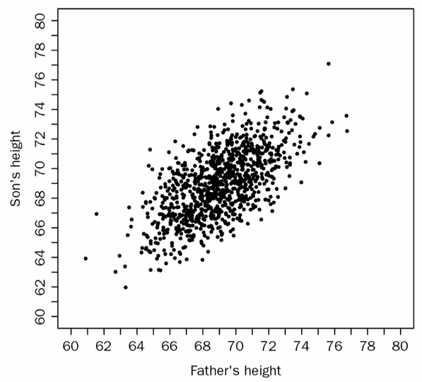
A British Eugenicist, Francis Galton, challenged this view by observing heritable traits such as height. One of his most notable findings was that while tall parents tended to have tall children, the children were not likely to be as tall as their parents. He demonstrated this by plotting the height of sons and fathers and on an x-y scatter plot and saw that the heights tended toward the average height. Regression to the mean is based on the fact that performance is often times a function both of random fluctuations or luck, and controllable factors or skill.
However, the controllable factors do not often contribute as much as it is thought to contribute and over time as the luck runs out, performance regresses to the mean value. Ellenberg goes on to demonstrate the presence of these effects in sports (the phrase “on pace for” is misleading as exceptional players early in the season will often regress to the mean) and weather patterns.
Limitations on correlation
Correlations are not transitive. If A and B are positively correlated, and B and C are positively correlated, A and C are not necessarily positively correlated. On first glance, this may seem both obvious and paradoxical. In order to understand it a bit better, Ellenberg considers the case of mutual fund investors. Suppose Laura has a fund split evenly between Facebook and Google. Tim’s fund is half GM and half Honda. Sarah has half Honda and half Facebook in her fund.
It is not unreasonable to expect Laura and Sarah’s funds to be positively correlated. The same could be said for Sarah and Tim. However, does that mean you can expect Laura and Tim’s portfolios to be positively correlated? No, you cannot. The non-transitivity of correlation is a problem that appears in many areas of life including medical research, politics, genetics, mutual funds and many other fields.
This makes medical research very difficult. For example, levels of high- density lipoprotein (HDL) are positively correlated with a lower risk of heart attack. However, that does necessarily mean that raising HDL by any means is also positively correlated with a lower risk of heart attack. It could also be the case, that some non-obvious factor is impacting both HDL levels and heart attack risk – this is analogous to the Honda stock affecting both Tim and Sarah’s portfolios.
If a drug intended to lower the risk of heart attack does so by raising HDL levels by means of the mystery factor then it may also reduce the risk of heart attack, but if it raises HDL levels by some other factor, then it is just shooting in the dark. This is one of the principal challenges in medical research. Understanding the difference between correlation and causation is crucial in understanding the relationships among various correlated variables.
This is why the phrase: “correlation does not imply causation” is so popular. But ultimately, these relationships can only lead researchers in the right direction and they have to directly test their hypotheses. If A and B are correlated, and B and C are correlated, test to determine whether A and C are correlated.
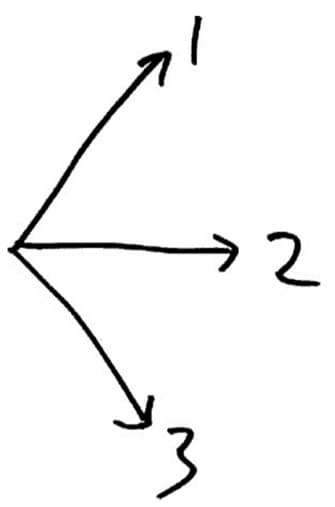
This same phenomenon can be observed in the world of politics. Rich states vote for Democrats, rich people vote for Republicans. This seems paradoxical: don’t rich people come from rich states? In the general case, the non-transitivity of correlation can be explained by Karl Pearson’s definition. While the formula itself is complex, it is helpful to think in geometric terms. Your set of variables can be thought of as an n-dimensional space, in which each set of variables corresponds to a vector. Under this geometry, the correlation between two points can be thought of as the cosign of the angle between two vectors. While you may not remember exactly how cosign operates, the only important things to know about cosign are that cos(0) = 1, cos(90) = 0, and cos (180) = -1. In other words, an acute angle (0 ≤ 𝜃𝜃 < 90) between vectors means there is positive correlation, a right angle (𝜃𝜃 = 90) between vectors means there is no correlation, and an obtuse angle (90 < 𝜃𝜃 ≤180) between vectors means they are negatively correlated. Once this definition of correlation is understood, it is easy to see how correlation is not transitive. In the graphic to the right, vector 1 and 2 are positively correlated (acute angle), vector 2 and 3 are positively correlated (acute angle), but vectors 1 and 3 are not positively correlated (right or obtuse angle).
PART 5: EXISTENCE
Majority rules systems only tend to work well when choosing between two options. For example, a 2011 Pew Research poll showed that while 77% of Americans wanted smaller government (that is, to cut government spending) when categorizing the government spending into 13 categories, the majority of respondents wanted to increase spending in 11 of 13 categories.
Only foreign aid and unemployment insurance – collectively less than 5% of spending – did not gain majority support. Some critics of the American public conclude that Americans just want a free lunch. A February 2011 Harris poll summarized this as “Many people seem to want to cut down the forest but keep the trees.”
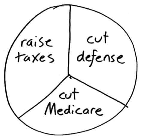
However, the issue is a bit more nuanced. Consider a simplified example in which a third of the electorate wants to raise taxes without cutting spending, a third wants to reduce spending by cutting Medicare, and another third wants to reduce spending by cutting defense spending. If you ask: “should we cut defense spending?” a majority of the country says no. Similarly, a majority disapproves of raising taxes and cutting Medicare.
So, while a majority of the country wants to cut spending, the majority is also opposed to cutting spending in any single category. The same divergence from a clear majority choice can occur in presidential elections. Consider the 1992 election where Clinton won 43% of the vote, Bush won 38% and Perot won 19%. A majority of the country voted against each candidate, but it still seems fair enough that Clinton won.
However, consider a possible circumstance: the 19% of Perot voters were broken down into 13% who preferred Bush over Clinton, and 6% who preferred Clinton over Bush. Now, if you were to poll the electorate 51% preferred Bush over Clinton. The presence of a third candidate, though no majority preferred him, may have changed the outcome of the vote. Here is a case where public opinion is tough to decipher, and a fair conclusion might be that public opinion does not exist in this case.
In order to address the paradox above, some democracies implement voting systems where voters can submit the first, second, third, etc. choice. This may seem like a fair system; however, circumstances arise that make it impossible to decipher public opinion.
Burlington, Vermont, one of the few US municipalities that employs instant run off voting (a voting system where the votes are counted twice, taking into consideration voters’ second preference), a different candidate is preferred based on how the votes are counted. Under the traditional American voting method, the Republican candidate would have won. Under the instant run off voting system, the Democratic candidate won.
If you consider all the preferences simultaneously, a majority of the voters preferred the Independent candidate over both the Democratic candidate and the Republican candidate; however, he did not receive enough first place votes to make it to the run off. Consider a simplified ballot count from the Burlington election. Under this count, a majority of voters prefer Montroll to Kiss; however, a different majority prefers Wright to Montroll, while a third majority prefers Kiss to Wright.
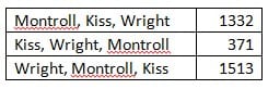
Who is the fair winner? Circles like this are called Condorcet’s paradox, named after the 18th century French Enlightenment philosopher Marquis de Condorcet. The conclusion here is that sometimes public opinion is impossible to decipher.
HOW TO BE RIGHT
How Not to Be Wrong: The Power of Mathematical Thinking paints math in a way that many (even most) people probably don’t think of it. Many of the computations that support the concepts that Ellenberg talks about are complex and out of reach to many people; however, his examples bring to light the usefulness and applicability of the underlying principles in everyday scenarios when we aren’t the ones performing the computations.
Given the title, it is only fitting that Ellenberg concludes with a summary of how to use the mathematical principals described in the text to always be right. However, the answer is not what many readers want to hear.
“Math gives us a way of being unsure in a principled way: not just throwing up our hands and saying ‘huh,’ but rather making a firm assertion: ‘I’m not sure, this is why I’m not sure, and this is roughly how not-sure I am.’ Or even more: ‘I’m unsure, and you should be too.’”
In other words, it is not possible to always know everything about nature, society or the outcome of the lottery; however, mathematics gives us a framework to uncover hidden structures, deal in the uncertain and make best guesses about everyday life that we can’t directly observe.
While mathematicians traffic in logic and rationality, purely deductive thinking is a dangerous proposition. F. Scott Fitzgerald once said: “The test of a first rate intelligence is the ability to hold two opposed ideas in the mind at the same time and still retain the ability to function.” As humans, we are not entirely rational beings, and this is a good thing.
A common piece of folk advice among mathematicians is that when you are working on developing a theorem you should spend some time trying to prove it correct, but also spend a significant amount of effort trying to disprove the very thing you are trying to prove.
This act of proving by day and disproving by night is valuable not just in mathematics, but also in other areas of your life including social, political, scientific and philosophical beliefs. If you can’t talk yourself out of your existing beliefs, you’ll understand a lot more about why you believe what you believe.
Ellenberg concludes his book with the following words, which do not need any further paraphrasing, summarizing or explanation:
“The lessons of mathematics are simple ones and there are no numbers in them: that there is structure in the world; that we can hope to understand some of it and not just gape at what our senses present to us; that our intuition is stronger with a formal exoskeleton than without one. And that mathematical certainty is one thing, the softer convictions we find attached to us in everyday life is another, and we should keep track of the differences if we can.
Every time you observe that more of a good thing is not always better; or you remember that improbable things happen a lot, given enough chances, and resist the Baltimore stockbroker; or you make a decision based not just on the most likely future, but on the cloud of all possible futures, with attention to which ones are likely and which ones are not; or you let go of the idea that beliefs of groups should not be subject to the same rules as beliefs of individuals; or, simply, you find that cognitive sweet spot where you can let your intuitionrun wild on the network of tracks formal reasoning makes for it; without writing down an equation or drawing a graph, you are doing mathematics, the extension of common sense by other means. When are you going to use it? You’ve been using mathematics since you were born and you’ll probably never stop. Use it well.”
Britt always taught us Titans that Wisdom is Cheap, and principal can find treasure troves of the good stuff in books. We hope only will also express their thanks to the Titans if the book review brought wisdom into their lives.